Assignment 4: Distance Azimuth Survey Methods

Introduction

Assignment 3: Report of Methods Related to Balloon Mapping Hardware Construction

Introduction

The intention of this assignment was to make preparations for two different projects. The first project is to map the UWEC campus mall using a camera attached to a balloon, much like the original methods used for remote sensing. The idea is to attach a camera rig to a balloon filled with helium and have it tethered to a person on the ground, who will be able to guide it around the campus mall area. The second project is a high altitude balloon launch (HABL). The HABL project consists of also attaching a camera rig to a helium balloon, but this will not be tethered to a person on the ground. The HABL will rise as high as it can, the balloon expanding as the atmospheric pressure decreases until it eventually pops, at which point the attached parachute will allow the camera rig to fall safely to the ground. Our assignment this week was to come up with the designs and determining the payload for each project.

Methods

Given the number of people in the class, it took a few minutes for people to decide what they wanted to work on and who else wanted to as well. I started off by verifying that the cameras we wanted to use had a continuous shot mode, as both projects could not be done without continuous shot.

Once we knew at least two of the smaller cameras had continuous shot, I moved over to assist with the construction of the balloon mapping rig. Our professor had purchased a kit online for a general guideline of a design we could use. Our professor also brought a large supply of seemingly random objects, though I believe that by the end of the day the majority of them had been used, or at least attempted to be used, in some way.

As we attempted to follow the directions (click link to see) provided by the kit, we quickly found out that we did not care for them, as they were slightly vague and the drawings were…interesting. This kit used a 2L soda bottle as the rig. We were to cut the 2L bottle in half and use string to create a cradle for the camera. After successfully taping the string to the camera to make the cradle (Figure 1) and pulling the top part through the 2L bottle, we noticed that the rig spun a lot, even just in a room. Another student thought of turning the 2L bottle horizontal in order to make it more aerodynamic and have more room for the camera. I decided to join the other student in researching the alternative design.

Figure 1:
Amy holding the camera from its cradle.  The pink string is wrapped
around the camera with tape applied to keep it from slipping off.

My partner and I began by taking another 2L soda bottle and cutting a hole in it large enough to fit the smallest camera we had.  We roughly drew a rectangle with a black marker on the 2L bottle and then used an exacto blade to cut it out (Figure 2).  Once the hole was cut, we then needed to determine how we were going to hold the camera in the bottle.  After a couple minutes of thought, we decided the best way to secure the camera was with zip ties.  So, we cut four slits above (or opposite side of) the hole for the camera that we could pull zip ties through (Figure 3).  We also cut two more slits on each end of the 2L bottle, trying to center them as much as possible, to slide zip ties through in order to attach the string that will hold the rig to the balloon.

Figure 2:
Kent (me) using an exacto blade to cut out the designated area
that the camera will be placed through.

Figure 3:
Stacy cutting the slits in the 2L bottle to slide the zip ties through.
There will be four zip ties total, two to secure the camera, and
two to secure the string that will be attached to the balloon.

After the slits were cut, we were ready to attempt placing the camera in and securing it to the rig.  It took several attempts to determine the best way to place the camera in, as we also had to get the zip ties around it and through the soda bottle in order to secure it.  We found the best was to hook the zip ties through and zip them slightly, then all we had to do was place the camera in the loose loops and tighten the zip ties.

Once we had the camera secured, we realized that since we were not as detailed as we should be for the final project, our camera was not perfectly centered in the rig, and this could cause issues with keeping the camera level, as the center of mass was not in a good location.  To counter this, we decided to make sure the string was an even length to both sides, and then tie a knot, resulting in a single loop at the top to attach the balloon (Figure 4).  This should keep the camera rig balanced.

Figure 4:
Stacy holding the camera rig, with camera in it.
The camera is secured by two zip ties, on each side of the lens,
meaning the only way the camera would potentially be able to
fall off is if the lens closes (which may be possible if the battery runs out).
Knot at top of string is to correct the center of mass and provide
single attachment point to balloon.

We are hoping the curved nature of the top of 2L soda bottles will substantially assist in the aerodynamics of the rig, and prevent it from spinning a lot.  As a precaution, we decided to add a vertical stabilizer anyways.  The idea is much like that of a wind vane (and vertical stabilizers on the empennage of aircraft), where you have a surface going vertical that will catch the wind, forcing the object to always face into the wind.  Since we did not have much for material, we used a section of another 2L soda bottle that was cut in half.  We cut four more slits on the aft section of the 2L bottle to place two more zip ties that will secure the stabilizer (Figures 5 & 6).

Figure 5:
Stacy using zip ties to attach the vertical stabilizer to the 2L soda bottle.

Figure 6:
The finished camera rig, with vertical stabilizer attached at aft (left side in picture)
section of the bottle.  We cut angles on the back so the stabilizer would not
interfere with the string attaching to the balloon.

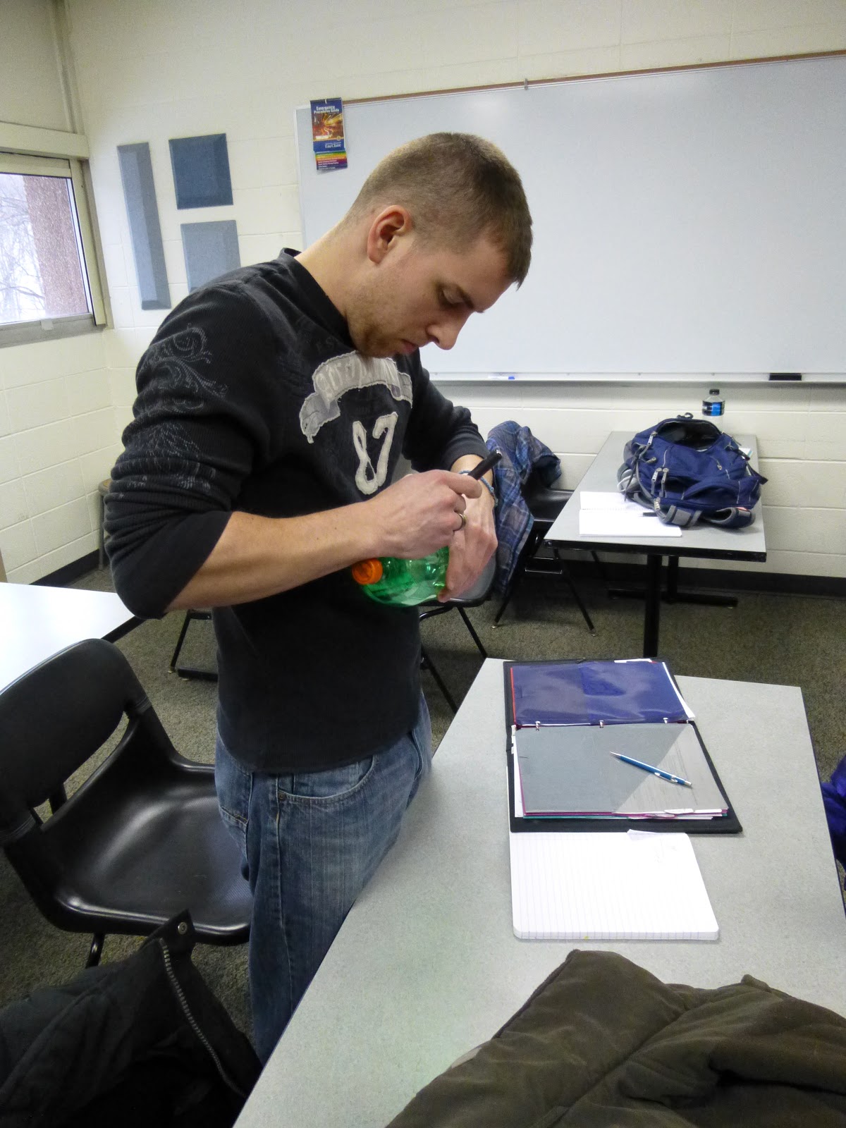
Given the blimp-like nature of our creation, we dubbed it the Hindenburg (do not worry, we will be filling the balloon with helium, not hydrogen).  With the camera rig complete, all we needed was a way in which to hold the button of the camera down to make it take continuous pictures.  The other group already had an answer for us, as they came up with the simple, but great, idea of tying a knot in the rubber band, and placing the knot on the button of the camera (Figure 7).


Figure 7:
We tied a knot in the rubber band, and placed the knot on the button
of the camera.  To put enough pressure on the knot, we had to twist
the rubber band around a second time.
This was not the camera we used in our rig.

Class finished as we were completing our rig, so I was unable to mingle with other groups to see how everything else was coming along.

Discussion

At the beginning of class I assisted in verifying that all of the cameras being used had continuous shot.  We found that all of them did, and they all worked well.  The only thing that could be improved with the cameras is if we were able to find one that was smaller, in order to help reduce the amount of weight on the balloon.

The group I was working with on the first design of the balloon mapper also deviated from the design in instructions that came with the kit.  They found that, with the camera they were using, a 2L bottle was not wide enough, so the only way the camera would be covered and protected by the bottle was if you forced it around, which was definitely not the desired result.  The group ended up switching to a cleaning solution bottle (Figure 8).  They used the same ideas as was in the instruction manual, using the cradle they already had to hold the camera up (Figure 9).  They then took a scrap from a soda bottle and taped it around the handle of the cleaning solution bottle to catch the wind and help reduce spinning (Figure 10).

Figure 8:
Cleaning solution bottle used to protect the camera.

Figure 9:
Cleaning solution bottle with camera being suspended by cradle.

Figure 10:
Cleaning bottle with piece of soda bottle wrapped around handle
and taped together.

As for the Hindenburg, I think our overall design is more aerodynamic, but that does not mean it will perform better.  It appears that we will be able to launch both designs, so it will be great to be able to see how each design does, and to see how much of an effect the design actually has.  One of the biggest concerns voiced with the Hindenburg, was the fact that the camera lens was so far away from the opening of the bottle.  To determine if this was an issue, we put the camera into continuous shot mode using the knotted rubber band method, secured the camera in the rig, and I walked around the room with it.  In figures 11 through 15 you can see my feet as I walk with it.  Much to our delight, there was no soda bottle in the picture.

Figure 11:
After securing the camera in the rig, I began walking around the room.

Figure 12:
Picture of floor as I walk around the room with the camera in rig.

Figure 13:
Another picture of floor as I walk around room with the camera rig.
There is still no view of the soda bottle, which is good.

Figure 14:
Final picture of me walking around room with the camera rig.
No view of soda bottle.

Figure 15:
In order to test that the camera was, indeed, secure, I swung it up to face the ceiling.
The camera neither fell out, nor did it even shift and show any evidence of the soda bottle.

As shown, the way in which we secured the camera to the rig did not result in any of the soda bottle being shown.  However, given the way in which we do secure the camera, there is the possibility that if we had it position slightly more forward or aft, a portion of the soda bottle may appear.  This is something we will need to test further in order to assure that in the actual launch we will not have issues.  We were also not very detailed in our design method.  Since we were mostly playing around with a new design, we didn't measure out exact distance, and we didn't pay attention to the center of mass.  When we make the final design, we need to make sure we are procedural and detailed in our methods.

Conclusion

I found this assignment to be quite exciting.  It was fun to work with a new group of people and experiment with new ideas.  Everyone seemed to work well together, and when new ideas were offered they were listened to and examine, not shot down.  Both of the balloon mapping designs were rather unique and came about in their own ways, and I look forward to seeing how they each develop and perform.



Assignment 2: Visualizing and Refining Our Terrain Survey

Introduction

This week’s assignment was to do a follow-up on the assignment from last week.  The intent was to examine the methods we used the week prior, and improve upon them to increase the accuracy of the terrain survey.  This second report is to be more thorough and detailed, providing a better understanding to the methods we used and a more accurate picture of what we accomplished.

Methods

To begin this week’s assignment, we loaded our x,y, and z coordinates from last week’s data collection into an Excel file, which was then loaded into ArcMap. With the points in ArcMap, we used the 3D Analyst toolbox to create terrain maps using five different interpolation methods, and can be seen in Figures 1-5. After the terrain maps were created, we then made a 3D rendering of them using ArcScene.

Figure 1:
IDW is the inverse distance weighted interpolation method.  IDW allows you to control how far away measured points are able to affect the interpolated point, allowing for smother or rougher surfaces depending on the power you set.  We used the default values during interpolation and there was no vertical exaggertaion in ArcScene.



Figure 2:
Kriging is a geostatistical procedure that estimates the surface based on a set of points.  Kriging looks at the statistical relationship of points, meaning it will predict a location’s values based on the measured values surrounding it. We used the default values during interpolation and there was no vertical exaggeration in ArcScene.




Figure 3:
The natural neighbors method interpolates points by drawing Voronoi polygons around all of the measured points.  A Voronoi polygon is then created around the interpolation point, and assigns a weight based on the percentage of overlap.  We used the default values during interpolation and there was no vertical exaggeration in ArcScene.

Figure 4:

The spline method minimizes the overall surface curvature.  It, essentially, takes a sheet of rubber and bends it through each of the measured points.  This provides a very smooth surface that mimicked our snow terrain effectively.  We used the default values for regularized spline during interpolation and there was no vertical exaggeration in ArcScene.

Figure 5:

A TIN is a triangular irregular network.  A TIN takes the input points (nodes) and draws lines to all the nearest neighboring points.  This creates many triangles, which also results in the terrain being very angular.  Before loading this into ArcScene, we had to convert it to a raster in ArcMap using ArcToolbox.

After completing the terrain maps and seeing the renditions of our prior week’s effort, it was obvious our data was not even close to the accuracy required for a good terrain map.  Whereas last week we used 10 cm x 10 cm grid system for our 100 cm x 230 cm flowerbed, we decided this week we would construct a 5 cm x 5 cm grid system.  It was cold last week, and it was even colder this week, which caused us to seek additional processes that would decrease our time outside.  One such creation was the use of a slide rule, as seen in Figure 6.  On top of the cold, our flower bed terrain was also covered in substantially more snow.  So, we had to do our best to create the same terrain as we had the week prior, which we believe we did relatively well.  Our etch marks from last week were still present, so it did not take us long to add the 5cm increment etches and pin up the y-lines.  With the grid setup complete, it was time to start collecting data.

Figure 6:
The slide rule laying across the flowerbed, with lengths of twine making up the y-axis.  Each twine is 5cm apart.

Rather than writing down the data points on paper and then having to type them into excel, we decided to have one person inside on a computer entering the data immediately.  I was the lucky person to be inside entering the points, while Amy took the x, y, and z measurements, and Joel relayed that information to me over the phone (Figures 7 & 8).


Figure 7:
Kent (myself) entering the coordinates into an
Excel spreadsheet.  Amy is taking the picture
while her and Joel were on a short break from
the cold.

Figure 8:
Amy (left) collecting the coordinates as Joel (right) relays
them to me via phone.

When the data collection was finally complete, much to Amy and Joel’s delight, we were able to immediately load the Excel file into ArcMap, run our preferred interpolation method (Spline), and render it in ArcScene.  Figures 9 shows the significant increase in accuracy of the terrain map.

Figure 9:
3D rendering of the spline interpolation method of our collected data. As can be seen, the terrain is
substantially more accurate and detailed (fine).  The same default values were used during
interpolation and there is no vertical exageration in ArcScene.

Discussion

Our methods during this resurvey of the terrain were substantially improved.  From the beginning we set ourselves up better than we did last week.  We made the decision that, given nature of Wisconsin weather at this time of year, we needed to remake the terrain, setup our grid system, and collect all of the data in a single session.  This can be difficult for our group, as all of us are both taking many courses and working at the same time.  The only day that we are really able to meet for two hours or more, outside of class, is Tuesday.  Last week we made the terrain during class on Monday, and returned on Tuesday to collect the data.  As can be seen in Figure 10, rain reduced our terrain in elevation considerable, and the frozen flowerbed made it very difficult to dig.  The use of the meter sticks as a moveable x-axis also reduced the amount of time it would take, as we did not need to place the 46 strands of string across the flowerbed.

Figure 10:
This image is from last week's data collection day.  It rained throughout the night,
substantially reducing and changing the elelevation of our terrain.

 

Deciding to have one person inside recording the data in Excel as it was being collected was also an excellent decision.  Last week it took me almost half an hour to enter the 291 points into Excel, and there were a multiple errors from typing mistakes, which required me to go back and correct them.  This time we had 987 data points, and the only issue was there were about 5 points that appeared to be missing. All I did was take a quick look at the attribute table, went to where the points should be, and found that I had copied the x coordinate too far down.  So, those 5 points were merely shifted over 5 cm and was an easy fix. 

The effect of our decision to use a 5 cm x 5 cm grid system is even apparent in just the data points when initially added to ArcMap (see Figures 13 & 14).  Figure 15 shows the end result of our improvised methods.

Figure 11:
Map export from ArcMap of our first week's data points.  These
were taken from a 10cm x 10cm grid system. There was a total
of 291 points.

Figure 12:
Map export from ArcMap of this week's data points. These
were taken from a 5cm x 5cm grid system.  There was a total
of 987 points.

Conclusion

Doing this assignment a second time was an excellent learning experience.  We were able to look back at what we did the week prior, improve upon our methods, and, in the end, create a significantly better map of our terrain.  Not only did we learn and improve our ability to collect data, import them into ArcMap, create maps of the terrain, and create 3D renditions of them in ArcScene, but we also came together as a group.



Assignment 1: Terrain Survey and Coordinate System

Introduction
The purpose of this experiment was to create a terrain, and then design and apply our own coordinate system to map the terrain. The underlying goal of the assignment was to force us to be able to conceptually capture topographic and locational data by creating a grid system and applying it in the field.

Methods
For the creation of the terrain, we used snow to form a miniature model of hilly topography in a raised flowerbed.  We molded snow into various geographical features, such as valleys, hills, lakes, and cliffs. The wooden sides of the raised flowerbed provided an excellent base for sea level; however, there was not enough snow to make the majority of the terrain above sea level, so we decided we would lower the sea level by a yet to be determined amount later on. We measured our flowerbed and found it to be 110 cm by 230 cm.  Given the amount of time we had, we determined that breaking the area into 10 cm x 10 cm grid cells would be the most efficient method of data collection.  We collected the x, y, and z coordinates at each vertex, with the southwest corner as our point of origin.  In areas we felt the topography was not being accurately depicted, we collected additional data.

Results/Conclusion
This assignment was an excellent precursor to actually going out in the field and collecting data.  It required us to examine the terrain we created and find a way in which to map it, without the use of GPS and other advanced methods.  Since this is my first time mapping an area, it challenged my visual/spatial thinking, and required me to learn how to apply a grid system to natural features.  We also learned the importance of planning ahead, the difficulties that can arise while working in the field, and the effect that could have on data collection, as we had built our snow terrain on one day, and came back the next to have it substantially altered by the rain.

As we completed the collection of our data points, we realized how coarse our map was going to be.  By using a 10 cm by 10 cm grid cell, we were unable to completely capture some of our features.  To rectify this, we collected additional data points.

Images:

Snow Terrain in flower bed (Day 1)

Beginning of Grid Cell Creation  (Day 2)

Completion of grid cells over flowerbed terrain (Day 2)

Data point collection (Day 2)