Assignment 12: Building An ArcPad Project and Deployment To The Field

Deployment of ArcPad to the field conducted on: April 29th, 2013

Introduction

With how many times we have been at the Priory, we have become quite familiar with the features and terrain.  This was quite evident during the final navigation exercise at the Priory, where most people never used their GPS except to set the waypoints for the markers they went to.  This exercise is an effort to begin a database with as much information as possible about the location, to assist with the restoration of the area.  We were provided a list of topics that could be examined, though we were suppose to limit the amount of overlap between groups in order to collect as much data as possible.  While providing us with experience, the data we collect can also be used in the future to create maps of the recently acquired Priory.  For this final exercise, we used Trimble Juno GPS units, loaded with ArcPad 10 software (Figure 1).

Figure 1: The Trimble Juno 3B GPS unit.

Study Area

For this exercise the study area was the same as all of our field navigation exercises, the Priory (Figure 2).  The Priory is a 112-acre hilly and mostly wooded plot just to the south of Eau Claire, Wisconsin.  It was acquired by University of Wisconsin - Eau Claire in 2011.

Figure 2: This map shows the study area found south of I-94 by Eau Claire, WI.

Methods

My group, again consisting of Beatriz and Joel, decided to map the trail markers and bench locations.  Before heading to the Priory, it was necessary to create a geodatabase, complete with feature classes that had domains.  Establishing domains is important when collecting data, as it can restrict entries to just a few options.  With domains created and applied to a feature class, when you are adding data points in the field, ArcPad will provide a drop down list of the available attributes.  If a range was specified for numeric values, then it will not allow you to enter values outside of that range.

With this in mind, my group began examining ways in which we could use domains to ensure integrity in our data on markers and benches.  For benches, we wanted to look at the condition, azimuth, proximity to the trail, and whether or not it was in a viewpoint.  For the markers, we decided to look at the color, shape, and medium. Figures 3 through 7 show the domains we created, their properties, and their coded values (if any).

Figure 3: This is the azimuth domain, which tells the
direction the bench is facing, and is limited to a value
between 0 and 360.

Figure 4: The condition domain describes the condition
of the bench, uses coded values, therefore limiting
the selections to Good (1), Fair (2), Poor (3), and Other (4).

Figure 6: The proximity domain is used to specify the
distance a bench is from the trail.

Figure 5:  The medium condition states what the sign is made from.  Since we were uncertain as to what all of the signs were, we came up with metal, flag, wood, and other.  It turned out most of the markers are metal, with the exception of trailheads.

Figure 7: The within viewpoint domain is a simple coded value of
yes (y) or no (n), used to specify if there is a particularly good view
from this bench.

With the feature classes and domains created in ArcCatalog, the remaining preparations were applying the domains to the respective feature classes, and then transferring the geodatabase to the GPS unit.  The domains were easily applied using the Assign Domain to Field tool.  In order to make the data ready for ArcPad, we had to enable the ArcPad Data Manager extension and toolbar, then merely click the Get Data for ArcPad button and follow the wizard.  Once the data was ready, I connected the Juno GPS and copied the files over.

Discussion

Once the ArcPad project was loaded onto the Juno GPS, the rest was fairly simple, though rather repetitive.  When we arrived at the Priory, we were immediately allowed to go and complete the tasks we planned.  My group immediately headed for the first trailhead that we were aware of.  Initially we started collecting each point together, with everyone filling in all the same information for the markers and benches.  After doing this for about 20 minutes, we realized that this was not an effective use of our time.  So, we came up with two options, either head of in different directions and collect everything we find (which would potentially lead to overlapping data, which would have to be sorted through) or we could split the work into three parts.  Up to this point, we only had four different items: triangle markers, benches, big circle markers, and small circle markers.  We decided to split it into three tasks.  Joel collected the triangle markers, Beatriz collected the benches, and I collected both sizes of circles.

Since we did not have a domain for the size of the marker, I used the notes field to tell when a circle was small; if it was large I left it.  In our efforts to collect all the data we could, and not knowing how many markers and benches their were, we were quickly separated.  At one point in the trip we came to a split in the path and had to choose which direction to go.  So, when the trail came back to the top of the open hill by the Children's Center, I navigated the same trail back down to the split, and took the other path.  I eventually met up with Joel, and we finished the last part of the trail.

With the data collected, we returned to campus and uploaded the data to our respective geodatabases.  Since merely copying all of the data over would result in some repeated data points due to us initially each collecting all of the data,  I used Select by Attribute to select all of circle markers, and exported them as a feature class to our group geodatabase.  I was then able to create the maps depicted in Figures 8 and 9.

Figure 8: Map of only the circle markers that I collected.

Figure 9: Map of everything collected by the group.

Conclusion


This exercise was pretty straight forward, but was still a great experience.  Being able to prepare a geodatabase for deployment in the field with ArcPad has many uses.  Not only was this experience using additional software, but the preparation requires you to start thinking about what issues you might encounter in the field, something that is very difficult to think about and accomplish successfully without actual experience.  Despite having been to the location three times, we hadn't been paying attention to the markers, what they were made of, and the conditions they were, so we had some limitations.  We had to design the geodatabase to not only work with what we knew, but to anticipate other issues that may arise.

Assignment 11: High Altitude Balloon Launch (HABL)

HABL Launch conducted on April 26^th, 2013.

Introduction

After two months of waiting for the proper weather, it was finally time to conduct our high altitude balloon launch (HABL). This year, winter weather decided to stick around a little longer than usual, and Friday, April 26^th was the first nice, warm day, with temperature reaching 72 degrees Fahrenheit. Despite having classes only on Mondays for three hours, our professor forewarned us to keep an eye on our email because he would email us the night before the launch, but he was expecting it to be Friday.

Method

The HABL consisted of three main parts. First was the large helium balloon, which allowed the camera to reach high altitude and take the video. Using 550 cord, the balloon was attached to both the parachute and the camera rig. Below the balloon was the parachute, which would be deployed when the atmospheric pressure reduced enough to allow the balloon to expand and eventually burst, thereby releasing the vertical tension on the parachute. The final part was the camera rig, which was just a styrofoam bait box, with a hole cut for the Flip Cam lens to be placed in for video recording. Also in the camera rig was a GPS locator, insulation, and several hand warmers to keep the box warm enough for the camera to continue operating. The FAA also requires that a strobe light be attached, so we attached one to the outside of the rig.

Figure 1: Our class heading to the campus mall area to release the balloon.
You can see the parachute connected to balloon.

We launched the balloon from the center of the University of Wisconsin – Eau Claire campus mall, shortly after 10:00 AM. Our professor was suppose to be able to see where the rig was via the GPS locator with either his iPhone or computer, however, for some reason he didn't receive the first update until almost 30min after the balloon was launched. Fortunately, about an hour and a half after the launch our professor finally received a signal from it, 78 miles to the east (Figure 2). When he asked for volunteers to go on the recovery mission with him, I volunteered along with fellow classmate Beatriz Viseau.

Figure 2: The is a map where the balloon was released (green) and where it landed (red).
Due to the some strong winds, it was pushed about 78 miles to the East/Southeast.

After stopping at the professors house to pick up some gear, we drove for about 1.5 hours to the expected owners house. The occupants turned out to be the owners of the land where the GPS signal was emanating from and were kind enough to give us permission to retrieve it. After about a one mile walk and navigating an extremely muddy field, our professor spotted the rig and parachute about 25 feet up in a tree (Figure 2). We had left the climbing gear in the truck, so our professor went back to retrieve it. When he returned, he began climbing the tree. Since the rig was stuck on the outer edge of a branch, we sent up a saw to our professor so he could cut the branch down (Figure 3). After about thirty minutes of sawing, our professor was exhausted, and the branch finally snapped, lowering our rig to the ground (Figure 4). There was much rejoicing (Figure 5).

Figure 2: Photo taken from the ground, looking up.  The rig was at least 25 feet up.

Figure 3: Professor Hupy grabbing the saw that we hoisted up to him.

Figure 4: The tree limb that was sawed off.  I attempted throw the rope into a higher
limb so we could hoist up a hatchet which would have made our professors effort a little easier,
but unfortunately he had it cut before I was able to get the rope high enough.

Figure 5: Professor Hupy holding the retrieved rig after cutting the branch and climbing back down.

With the rig successfully retrieved, we packed our things and made our way back to Eau Claire.

Discussion/Conclusion

The following images are single frames from the video. Unfortunately, the Flip Cam had a 1 hour limit on video recording time, resulting in only part of the descent being filmed. The Go Pro was the most desirable, and will likely be the camera used in the future, but it was not obtainable for this event.

The following stillshots extracted from the video show some of the amazing footage that was obtained.  Unfortunately, as the rig gained altitude, condensation began forming on the camera.  In future launches, the condensation buildup may be able to be reduced by placing rice in the rig as well.  Even with the condensation, the footage was still amazing.

Figure 5: Stillshot of the video as it follows the Chippewa River.

Figure 6: Stillshot as the balloon continues to gain altitude.

Figure 7: Some intense upper atmospheric winds allowed the camera to catch
glimpses of the curvature of the Earth.

Figure 8: Another glimpse of Earth's curvature.

Figure 9: The tops of some clouds were caught as well.

Despite having seen many images similar to these, most of them being higher quality and not having a giant circular blur in the center, it was still extremely satisfying and inspiring to be a part of this exercise.  I look forward to doing this sort of project on my own in the future.

Assignment 10: Aerial Mapping with Balloon I and II

Balloon Mapping I conducted: April 1st, 2013.
Balloon Mapping II conducted: April 8th, 2013.

Introduction

Back in February we began the preparations for doing both aerial mapping with a balloon and a high altitude balloon launch.  The weather is finally beginning to resemble something like Spring, and so we are finally able to begin the aerial mapping of our campus.  This was a collaborative effort, and a learning experience for everyone, as nobody in the class, including the professor, has done aerial mapping with a balloon, nor georeferenced and mosaicked the imagery that resulted from such an endeavor.

We conducted balloon mapping on two different occasions.  The first event took place on April 1st, and was more of an experimental day to ensure everything was in working order and to work out any potential issues.  On April 8th we went out the second time, with great success.

Since I will be discussing both days in this single blog post, I will first examine the events of April 1st, then the events of April 8th, followed by a comparison of the two days in the conclusion.

Balloon Mapping I

Methods and Discussion

Upon arriving at class, everyone was instructed to split into groups and accomplish particular tasks.  Some were needed to fill the balloon with helium, others were to ready the camera rigs, and another group needed to measure and mark the balloon string so we would know how high the balloon was.  I worked with the group marking the balloon strings.  The professor had us mark every 50 feet, up to 400 feet (Figures 1, 2).  Each 50 was marked as black, each 100 was red, and the 400 mark was green and red.  These marks were intended to provide us with an idea of the height reached by the balloon.

While I was helping mark the balloon line, another group found a unique way to transport the large, heavy helium bottle from the second floor storage room, to the garage where the balloon was to be filled (Figure 3).  Once the lines were marked, we headed down to the garage to deliver the string and see how the filling of the balloon was going (Figure 4).

Figure 1: Amy and myself holding the string taut so I could mark it.
Amy walked the string back and forth while Beatriz and I marked it.

Figure 2: An example of a marking we made.  Red was used to
represent 100, 200, 300, and 400 feet (though 400 also had green).

Figure 3: An unconventional, but unique and effective way of transporting
the large, heavy helium bottle.

Figure 4: The filling of the balloon.  

When we arrived, they were finishing up with the filling process, and attached the string to the balloon.  With the string attached to the balloon via a metal ring and carabiner, and an eTrex GPS unit as well, we headed to the campus mall where we would launch the balloon.  Last minute checks were made to verify the was set to continuous shot mode and that pictures were being taken.  The styrofoam enclosure was then taped shut and the balloon was released (Figure 5).  As can be seen in Figure 6, the wind was very strong, and immediately pushed our balloon to the East, restricting its ability to gain altitude.  After walking it around the campus mall, it was reeled in and we returned to the garage to attach and test the HABL rig.

Figure 5: Professor Hupy attaching the eTrex GPS unit to the balloon before it
is released.

Figure 6: Picture of the balloon in the sky.  Though it is somewhat difficult
to tell, the balloon is pushed very far away and is not actually that high up.

With the HABL rig attached, the balloon was released in the campus mall area.  The class, eager to get some interesting pictures, decided to walk it over the bridge towards the Haas Fine Arts building.  Due to the strong, prevailing winds, the rig was being whipped around substantially, and at times the balloon was even being contorted (Figure 7).  The wind eventually caused the string to snap, resulting in the balloon rising, and the camera rig falling towards its untimely death (Figure 8).  With the class watching in horror, the rig splashed into the river, and everyone was suddenly glad the camera was in a waterproof case and the rig was intended to float.  Fortunately, not only did the rig land in the water, but it also landed towards the outside of it, resulting in it being pushed relatively close to the shore.  Our professor quickly navigated the snow covered, rocky slope to the rivers edge, grabbed a tree branch, and managed to snag the rig in a single thrust.  With rig in hand, our professor returned to a crowd of relieved students (Figure 9).

Figure 7: In this image you can see the balloon, rig, and string.  This image allows for
you to tell how far behind the balloon is from where we were walking.  The image may need
to be enlarged to see the string and rig.

Figure 8: The escaped balloon can be seen rising into the air.  Again, the
image may need to be expanded to see it, but it is directly above Hibbard (tall red brick building),
and in the middle of the gradient from light blue to dark blue sky.

Figure 9: Professor Hupy climbing back up the slope after grasping the
rig from the Chippewa River.

After returning to the classroom, our professor uploaded the photos from the first launch, along with the video from the second.  Figure 10 through 12 show some of the images obtained from the Lumix camera used in the first rig.  While a few of them turned out really well, most of them were unusable due to the angles or blurriness.

Figure 10: One of the usable images obtained. This is the campus mall area where
both balloons were launched from.

Figure 11: Thanks to the wind, the camera captured a cool image of both
the walking bridge and the Chippewa River.

Figure 12: Again, the wind provided an excellent photo of the new
Davies Student Center, and parts of upper campus.

Balloon Mapping II

Methods and Discussion

For this class period, the class split into the same groups in order to accomplish the tasks quickly, providing as much time as possible for mapping.  One new group was formed to take three different GPS units and collect ground control points for use in the mosaicking process.  As for the string, this time our professor wanted to increase its measured length so it could be allowed to go even higher.  We marked increments every 50 feet, up to 700 feet (Figure 13).  This time, the rig was merely a string cradle for the camera, with an arrow strapped to it and a fin attached (dubbed 'camarrow').  The arrow and fin act as a wind vane, pointing the camera in the direction of the wind, thereby increasing stability.  With the camarrow attached to the balloon (Figure 14), we headed to the campus mall, where it was quickly examined and then released (Figure 15).

Figure 13: Again, Amy is walking with reel of string while Beatriz and I hold the string
at opposite ends. This time we increased the range up to 700 feet, with increments every 50 feet.

Figure 14: The "camarrow" on its journey from the garage to the campus mall.
As you can see, the arrow is strapped to the camera using zip ties, and has a large
fin attached to it.  The allows the arrow to act as a wind vane, increasing the stability.

Figure 15: Professor Hupy assisting in the release of the balloon, after
students verified it was in continuous shot mode and was taking pictures.

The combination of having only a light wind and fin substantially improved the stability.  The lack of wind also allowed the balloon to rise mostly straight up.  The balloon was walked around a good portion of lower campus, and then taken across the bridge, around Haas, and into the parking lot between Haas and the Human Sciences and Services building.  As we were following the sidewalk back towards the bridge, we realized it was a bit risky to walk it with the balloon up, as several substantial tree branches reached close to Haas, making it a tight squeeze.  We decided to play it safe and reeled the balloon in to transport it back over the bridge (Figure 16).

Figure 16: A group of us helping unravel the twisted string as it is reeled in.
The balloon was brought down across the river by the parking lot by Haas.  We then
walked it across the bridge and released it back in the air upon reaching the other side.

As we were reeling it in, we counted the marks and found out the balloon had been over 500 feet in the air.  We then carried the balloon over the bridge, releasing it again once we were on the other side of the river.  We proceeded towards the hill to upper campus, taking the stairs once we reached it, and then walked to the big field next to Towers, which is where we reeled it in the final time.  This day's mapping resulted in 4846 images.  Figures 17 through 23 show a few of these.  Some of these images were then used to construct mosaics, as discussed in Assignment 9.  Unfortunately the collected ground control points were unusable due to their level of inaccuracy.  The professor intends to have students use Total Stations in the future to collect accurate GCPs.

Figure 17: Image of the Student Center (Center), McIntyre Library (upper right),
Schofield (lower right), and part of the new campus mall area.

Figure 18: Image of the walking bridge over the Chippewa River.
The single building depicted is the Haas Fine Arts center.

Figure 19: After walking around Haas and through the parking lot, we
began reeling the balloon in.

Figure 20: The balloon was released again upon returning to the lower campus
area, where we then headed towards upper campus.

Figure 21: We climbed the stairs to upper campus.  In the image are Hilltop (on left over road),
Horan Hall (Center), and Governor's Hall (Right).  A small portion of Towers Hall can be seen
in the upper left corner of the image.

Figure 22: This image was as we headed towards the large open field next to Towers Hall.

Figure 23: The balloon is now over the field next to Towers Hall (bottom).
The sand volleyball, tennis, and basketball courts can also be seen.

Comparison and Conclusion

Both balloon mapping exercises were an excellent experience.  Everyone learned a lot and most, if not all, thoroughly enjoyed it.  The first exercise turned out to be mostly for working out the kinks, which was definitely needed.  With it being everyone's first time, it's unlikely for everything to go smoothly, and complications were expected.  The wind was particularly strong the first time, which we now know from experience that it can greatly impact the outcome.  With winds as strong as they were, a kite would have been more useful, and our professor intends to look into them for future classes.   An accurate set of ground control points are definitely important to assist in the georeferencing and mosaicking process.

There were substantial improvements across the board in the second exercise.  With the same people performing the tasks, they were completely faster, allowing more time for collecting imagery.  After seeing the effects of the wind in the first exercise, we realized the necessity to increase stability as much as possible, leading to the concoction in the second exercise that worked very well.  Whereas in the first exercise about 320 images were collected and a video, the second exercise resulted in 4846 images.

Overall, I found the balloon mapping exercises to be very useful and fun as well.  I can see many useful applications for this cheap method of obtaining high resolution imagery.

Assignment 9: Georeferencing and Mosaicking

Georeferencing and Mosaicking conducted between: April 8th and April 15th, 2013.

Introduction

This week's blog post will discuss the georeferencing and mosaicking process that took place after obtaining aerial imagery from a balloon mapping rig.  Explanation and discussion of the balloon mapping process will be posted in a blog next week.

Through the balloon mapping process we obtained nearly 5000 images of the University of Wisconsin - Eau Claire campus.  Very few of these images were selected for the mosaicking process, as some of the images were blurry or excessively similar to the other images, as photos were taken every second.  The campus was broken into six areas, one for each group in the class, with three students in each group.  It was then up to each group to georeference images in that area and create a mosaic.  Each group would then place their mosaic in a geodatabase for everyone to access.

Georeferencing

Before beginning the georeferencing process, there are a couple bits of information that are necessary to understand.  First, is the RMS error. The error, as described by ESRI in the ArcGIS Help file, is the difference between where the point ended up as opposed to the actual location that was specified.  The total RMS error describes the consistency of the transformation between control points, with greater consistency as you approach 0.  This does not mean that a georeferenced image with an RMS error of 0 is perfect, as the accuracy is dependent on the control points, and, therefore, if poor control points were selected then accuracy may still be poor.

Another important factor in georeferencing is the use of transformations.  A transformation allows a raster dataset to permanently match the map coordinates of the target data, and there are multiple options to chose from.  My group chose to use a second-order polynomial transformation, as this seemed to provide the most accurate image.  A polynomial transformation is built on control points and a least-squares fitting (LSF) algorithm.  The LSF algorithm intends to derive a general formula that can be applied to all points, which often results in slight movement of the control points.  A second-order polynomial transformation requires at least 6 control points to use.

The best way to georeference images would be to have ground control points taken with an accurate GPS.  A few members of our class did this while everyone else was with the balloon.  However, at the time of data collection the group was unaware that the balloon would be going to upper campus, and so ground control points (GCP) were not collected there, which is the area my group was designated for georeferencing and mosaicking. (In the coming weeks we may use a Total Station to obtain ground control points on campus.)

For the time being I will be using a reference image and using objects in the image, such as sidewalks, pavement, and intersections, as control points.  In Figure 1 you can see some of the points I used to georeference the image.  As can be seen, buildings would be difficult control points to use, since the angle of the camera greatly affects how much of a building you can see.  This makes the mosaicking process particularly difficult at times when you are trying to put images together that have varying angles of the same building.

The georeferencing itself is rather simple.  Merely click the add control points button on the Georeferencing toolbar, then click a spot on the map where a control is desire, and then click that same spot on the reference image.  Each control point made shows up in the Link window, showing the RMS error for each individual control point created.  Once all of the desired control points are created and the image is satisfactory, the information can be saved with the image by clicking on georeferencing and selecting Update Transformation.  Alternatively, the image can be rectified, which creates a new image and permanently applies the transformation to it, which is what I did.

My first time going through my chosen images and georeferencing did not go over quite so well.  For some particular reason I was not thinking clearly and I used the tops of buildings in the balloon image and referenced them to the tops of the buildings in the reference image.  As is likely obvious to those reading this, that is a very poor method to use.  This may be fine if the image is from directly above the building, but in our images only Hilltop (the building that goes over the road) could be used for this.

Figure 1: This is the first image I georeferenced, corrected and not using the tops of buildings for control points.
The red circle on the image shows where the Total RMS Error is located.  The red line delineates
the transformation method used.  All of the control points can be seen in the image, represented
by the green and red crosshairs with a number above them.  

As shown in Figure 1, I used 18 control points for the image, which is three times the number required for a second order polynomial transformation.  Though only six are required, earlier on I managed to obtain a total RMS error of around .5 using only six control points, but the image was way off.  I found that my best images had between 12 and 20 control points, and I would recommend at least 12.

Figure 2: The second image I georeferenced.  Again the RMS is circled and the transformation is
underlined.  The image is really far off on the top right, but that was intentional.  For this image I
focused the accuracy at the bottom of the image, as this one will be underneath when mosaicked. 

I was in a hurry when doing the mosaicking and forgot to take screenshots of the other four images used in the mosaic, but the process was the same.  I tried to ensure that each image had at least 50-60% overlap, and each one focused (was most accurate) on a different area.



Mosaicking

The mosaicking procedure was relatively simple as well, yet somehow managed to turn into a pain, as there seemed to be issues, either with the server or with my ArcMap session (or perhaps me).  To mosaic the images, I simply ran the Mosaic to New Raster tool.

Figure 3: These are the settings I used when running the Mosaic To New Raster tool.

Yet again I failed to take screenshots, this time of the errors/issues that occurred.  Hopefully I will learn from this and remember that whenever I encounter an error message or the result is not what is expected, I will take a screenshot for proof, discussion, and potentially determining the reason for the error.

The mosaic of my images can be seen in Figure ?. There are several discrepancies with my mosaic.  One is that the rope can be seen in multiple images.  Given the number of images we obtained, it is definitely possible to use enough images to not have the rope in the image; however, it would take me a considerable amount of time, of which I have been unable to find.  Hopefully in the near future I will be able to return to the images and create another mosaic without the rope.

Figure 4: My mosaic based off of four images.

While I was mostly covering the road up the hill, Horan Hall, and Hilltop, my group members were focused on the other areas of Upper Campus.  Once each of us finished our individual mosaics, we then mosaicked all of ours together, to be placed in an open geodatabase for the whole class to access.

Figure 5: Our group mosaic of Upper Campus.

Conclusion

While the process was interesting at first, it grew tedious towards the end.  This may have been partly due to the fact that I realized the mosaic would not (and did not) turn out as great as I had hoped.  Given the amount of imagery I think it could certainly be done much better, and hopefully sometime in the near future I will have the time to come back and try again.  It also would have been more enjoyable had there not been repeated issues with the creation of the mosaic.  As is likely apparent after reading this post, this particular assignment was challenging in spots, and I hope to be able to come back to these images and turn them into a better mosaic.

Assignment 8: Navigation activity using GPS and Map

Exercise conducted on: March 25th, 2013.

Introduction

This blog post discusses the final navigation exercise and compares it with the prior three weeks. This week the field experience was a bit more intense, mostly due to the incoming fire. While combining what was learned over the last few weeks in navigation, we were also provided paintball guns to combat the other teams. The goal for this week was to collect as many of the fifteen points as possible, in any order. We were in the same groups as before, making six teams total. The weather finally decided to cooperate, as it was sunny and in the upper 30's (Fahrenheit), though there was still a substantial amount of snow on the ground.

The Methods section of this post will discuss the events of this week. In the Discussion section I will compare the experience of this week with the past ones, recap what was done in the three prior weeks, and discuss the important items learned.

Study Area

The area of interest in our field navigation exercises has remained the same over the last three weeks. The exercises were conducted at the Priory, a 112 acre, mostly wooded area purchased by the University of Wisconsin – Eau Claire in 2011, and located just outside of Eau Claire, Wisconsin. The monastery located there is now a daycare and nature center for children.

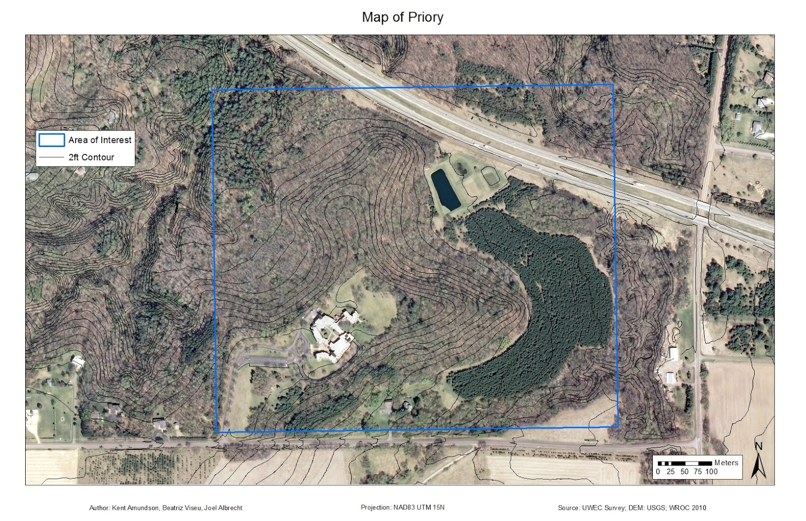
Figure 1: Map showing the area of interest at the Priory.  All course points are within this boundary.

Our professor created three navigation courses on this property, with some overlap in them to make it more difficult and ensure students are using the proper methods to find the markers (Figure 2). Each course consists of five points with an orange and white marker at each point.

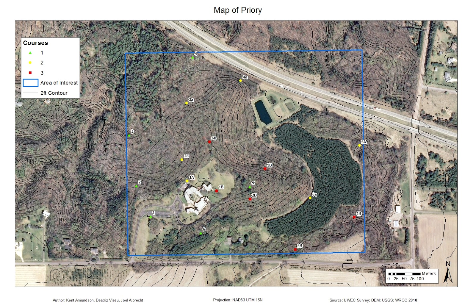
Figure 2: Map showing all of the course points and the course they belong to.
The area of interest is included as well, for reference.

All exercises took place in the month of March, which in Wisconsin can have quite variable weather. This year the weather was bleak, as we multiple snow storms and for the most part the temperature remained below 40 degrees Fahrenheit. The snow storms seemed to always come on the weekend prior to our Monday expeditions. All three times that we were at the Priory the snow ranged from ankle to knee deep, so wearing the proper clothing was necessary to stay warm (Figure 3).

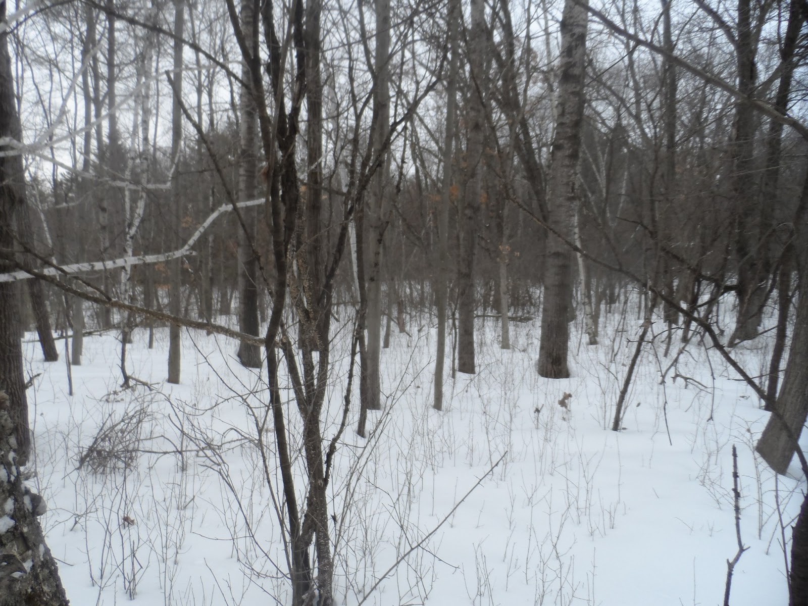
Figure 3: The snow covered terrain that we had to navigate all three weeks.
It ranged from ankle deep in some spots to knee deep in others.

Methods

We arrived at the Priory to see 18 Tippman A-5 paintball guns lying on the pavement with full hoppers and CO2 (Figure 4). We were each instructed to grab a gun, a mask, and fire off a few shots to get a feel for the gun for those who haven't paintballed before, which was only a couple people. Snowshoes were also available to those who wished to use them. I chose not to since we were paintballing, as I didn't want to be restricted on movement and I felt they would limit my agility. Each person was also carrying a Garmin eTrex GPS unit, again. We were instructed to keep a track log (set to take a point every 30 seconds) and to mark a waypoint at each marker. The paintballing rules were that if any member of your team was hit, the whole team had to sit out for 2 minutes. Also, we were required to stay away from all buildings and open areas, as is shown on the maps we created for this week (Figure 5).

Figure 4: The Tippman A-5 paintball gun.

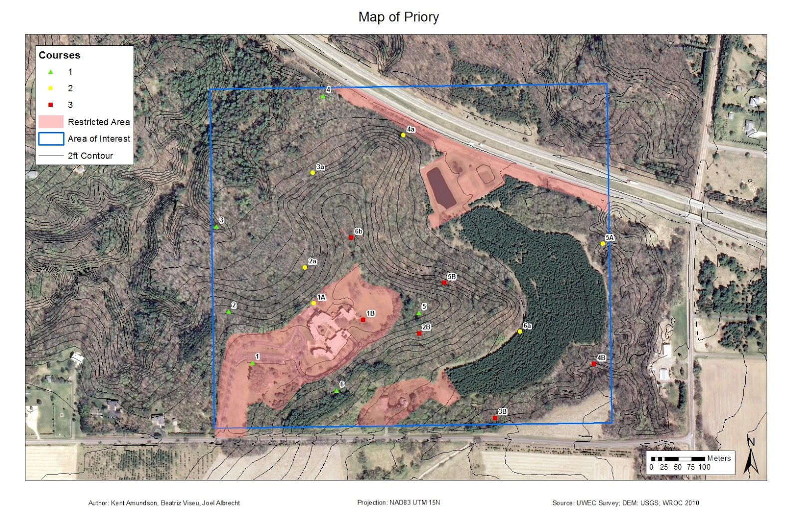
Figure 5: Map of the restricted areas, in relation to the course points and area of interest.
The top one was restricted due to visibility from highway.  The left area was due the presence
of many small children, and the area on the bottom center was a private residence.

My group decided to head for the points on course one and two first, as they were closest to where we were starting. There was a five minute no shoot at the start so that there wasn't a ton of shooting right around the starting area, which allowed us to get the first point with no issues. Shortly after leaving the first point we heard shooting slightly to the southwest of where we were heading. We headed straight for the marker in the ravine that we had issues with during the first navigation exercise. As we approached we saw that another team was across from us standing on the other ridge. After about five minutes of shooting back and forth we made a truce. It was difficult to hit anyone with all of the brush around, the paintballs kept breaking on the branches. Given the steepness of the ravine, it was decided that I would take both Joel and Beatriz's GPS units down with me so I could mark the waypoints, while they stayed on top to provide cover fire if necessary. I then slid down into the ravine and proceeded to mark the points. Just as I was finishing, Joel shouted down to me that another group was coming towards us. I decided to follow the ravine a ways so that I wasn't sitting in the open for the other team. While the ravine was fun and easy going down, it was quite the opposite on the way up, especially when two members of the other group spotted me on my way up. Luckily our professor had the PSI turned up on the guns, as this made the guns even more inaccurate at longer ranges. I took cover behind trees when necessary, but I was able to make my way back up in bursts. Once I regrouped with my team we headed on to the next points, keeping an eye on our backs for the other team.

As we continued on we gathered more points and had a few more skirmishes. Unfortunately, the masks we were using kept fogging up, which was rather frustrating at times and heavily limited sight. Towards the end of our exercise we saw two groups fighting each other and decided we wanted to flank them and see how much damage we could do. As we made our way towards them, someone spotted us and two of them broke off to engage us. After a short firefight, some of us ran out of ammo while others realized how low they were, so we formed a 9 person group and began heading back towards the starting point since it was getting towards the end of our time.

After the exercise, we had to upload our track logs and waypoints into ArcMap and place them in a public folder for everyone to access and create maps with, again. Figures 6 through 8 show the maps I created of the exercise. When looking at just my track log in Figure 6, you can see the locations that firefights occurred, as there are many dots in a small area.

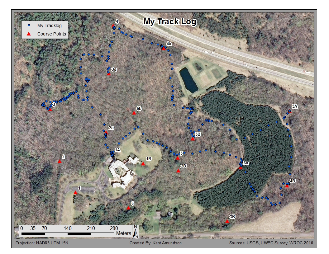
Figure 6: This map depicts the path I was took in navigating the course markers.
Areas with a greater point density are where shootouts occurred.

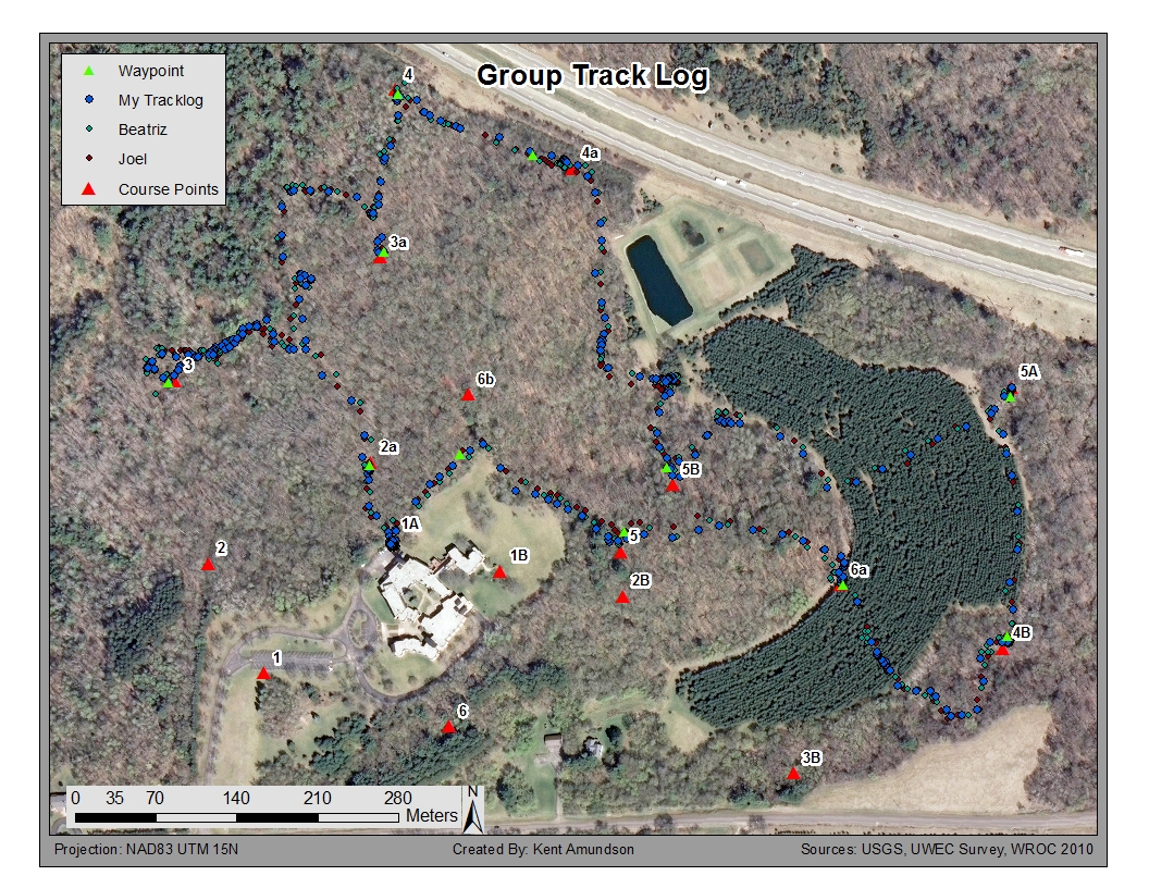
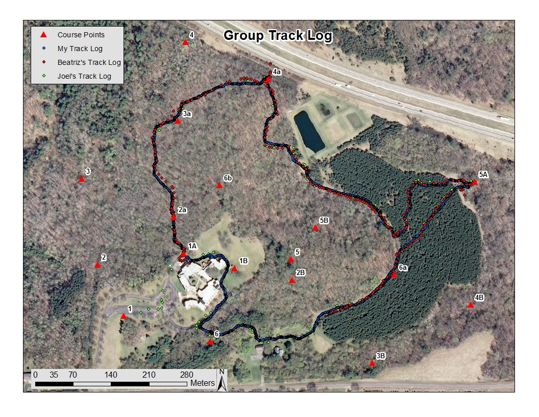
Figure 7: This map shows the track logs of all three group members.  Since I was carrying all three GPS
units after the first encounter, differences in position are mostly due to the positional accuracy of the
GPS unit, along with the track logs being started at different times.

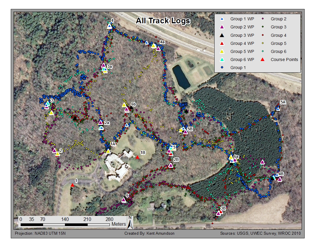
Figure 8: This map shows the track logs and waypoints collected by each group.

Recapping Prior Weeks

Week 1

During the first week of our land navigation exercise we created a topographic map (Figure 9) using ArcMap and established a pace count, both to be used for the second week. All of the following data was provided for us by the professor: a digital elevation model (DEM) obtained from USGS, orthographic images obtained from the Wisconsin Regional Orthophotography Consortium (WROC) in 2010, and two foot contour lines that were surveyed by UWEC during the purchase of the Priory.

The pace count was merely walking in a straight line for 100 meters and counting how many times you step with your right foot (starting with your left foot). We did this three times to determine consistency, and the best person was to be the pace counter for the exercise in week two. The counting would be slightly different at the Priory, given the change in elevation, but for our purpose this was relatively minor.

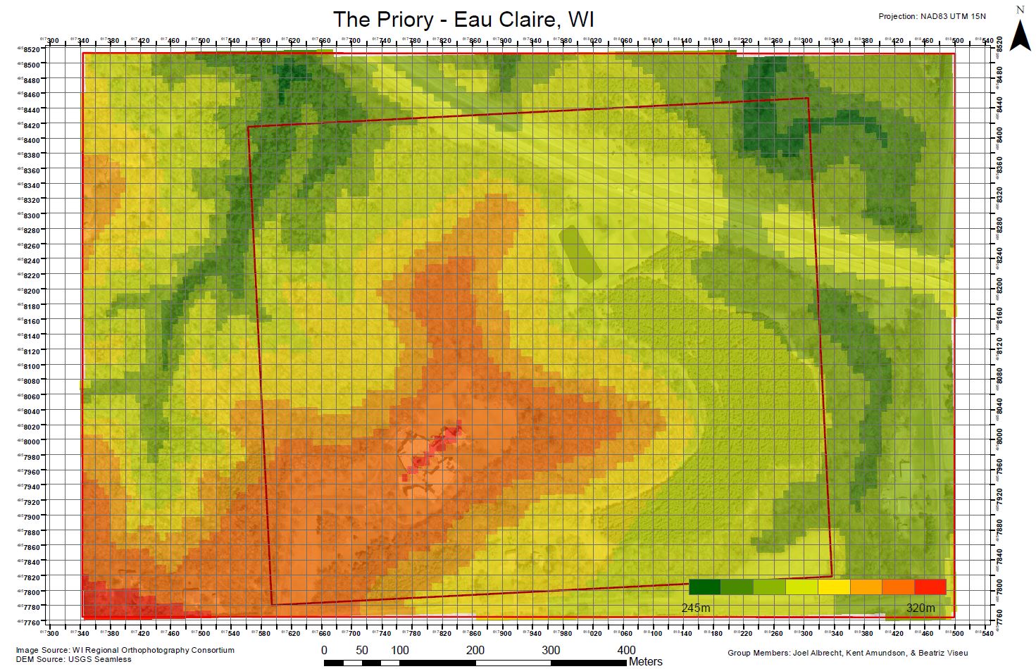
Figure 9: This is the map chosen by our group, for use during the first field navigation
exercise conducted at the Priory.

Week 2

The second week of our exercises involved navigating the Priory with a map and compass. The map we created was printed and course marker locations were given to us in UTM coordinates. We then plotted those points on the map and received a short briefing on how to use the compass and how to determine bearing. Once the briefing was completed, we found the bearings to get to each point and headed outside to start the course.

This week was particularly frustrating for my group. While we found the first point with no issues, the second point tricked us. We did, however, learn an important lesson: always trust the compass. While the point didn't look like it was down in the ravine on the map (due to not using the 2-foot contour lines), it was, and had we just continued following our compass down we would have seen it. We spent at least 30 minutes searching for the point before our field supervisor found us and moved us onward.

Week 3

In the third week we used a Garmin eTrex GPS unit to navigate another course at the Priory. Again we were provided UTM coordinates for the markers, only this time on a different course. This time the navigation was quick. Initially we paid close attention to our UTM coordinates on the GPS, and walked in the direction that would make the numbers get closer to those on our sheet. After the second point, Joel found out how to create a waypoint with the GPS, which then displayed an arrow on the screen in the direction we needed to go and the distance we needed to travel. The course was easy from then on, with the exception of the terrain and snow up to our knees. We completed the whole course in just over an hour, which is about how long we spent on just two points in week two. With track logging on our GPS unit we were able to create a map showing the path we took (Figure 10).

Figure 10: This is my group's track log for week 3's course navigation.

Discussion

This week's exercise was definitely the easiest, mostly because we hardly needed to use our GPS or map to find the markers. Since this was the third time we had been in the field, we knew the first two courses and the point locations quite well, so the only time we really needed to use our GPS was for the points on course three.

These land navigation exercises were an excellent learning experience. Not only did I acquire new skills, but I also learned from the mistakes that were made throughout these four weeks. In the first week my group found out the importance of trusting your compass. Had we trusted it, we would have found the point much quicker, and would have been able to move on and collect more points. We chose to trust our map more, but unfortunately the DEM used to create the map wasn't made with a low enough interval. This resulted in the marker appearing as though it was on or near the ridge. When looking at a map that used 2-foot contour lines, it was obvious that the flag was in the ravine.

Another important lesson learned was how the compass, when used properly, can be just as accurate (if not more so) than a GPS. The positional dilution of precision (PDOP) can be affected by canopy cover, buildings, and the atmosphere. Given that we were in a forest, the PDOP could vary. We were in this area in winter, when there is little canopy cover. In summertime, when the trees are in full bloom, the PDOP would likely be reduced due to the increased cover. Despite navigation by compass being much slower, it is always a good idea to carry a compass, just in case your GPS battery dies, or worse.

Conclusion

While navigation by map and compass is by far the slowest, it can still be fun and a good secondary option in case of equipment failure. A map with satellite imagery and contour lines can give a good idea of the type of terrain that will be covered, allowing for more suitable paths to be found, and also show landmarks and vegetation of the area. Even though paintballing was mostly just a fun addition to the exercise, it also required people to be pay closer attention to their surroundings. When using the GPS, it was easy to just put a waypoint on the GPS and walk in the direction of the next marker. With everyone armed, it encouraged people to constantly be looking around, taking in the environment.

As can be seen, these exercises have produced multiple skills and experiences that can be applied to both a professional career and outdoor hobbies. This post brings an end to the land navigation exercises conducted over the last four weeks.